Black to play
Black captured
0
White captured
0
Moves
Also called Weiqi, Baduk. Surround territory; capture what cannot live.
Handicap stones are placed for Black, White moves first, and komi drops to 0.5.
A Monte Carlo Tree Search engine, guided by a Neural Network for move ordering.
The whole opponent is one loop, repeated until its clock runs out. Each pass has four steps:
Run a few thousand times, this grows a tree that is deep along lines worth thinking about and shallow everywhere else. The move played is the one visited most.
UCT is the rule used in step 1 to decide which move to look at next. Each candidate is scored:
where n is how often this move has been tried, w how many of those were wins, N how often the position above it was visited, and C a tuning constant. The left term is what we know; the right is what is still unknown — the width of the uncertainty around that win rate. A move is ranked not by how good it looks, but by how good it could plausibly still be.
That balances trying new moves against pressing good ones: a move tried twice carries a wide bonus and gets another look, while one tried a thousand times must earn attention on its record. Because the bonus grows with ln(N), a move starved early is eventually revisited — which is why UCT converges on correct play given unlimited time.
UCT alone is far too slow here. With up to 361 legal moves, each needs on the order of a hundred simulations before its win rate means anything — tens of thousands of games just to form a first opinion. RAVE buys that time back using an observation about Go: a good move is usually good whether you play it now or ten moves from now.
So when a random game finishes, every move that appeared anywhere in it is credited as though it had been played first. One simulation updates a hundred estimates instead of one. That estimate is biased — sometimes timing is the entire point, as in ko fights, ladders and capturing races — so it is blended with the honest UCT figure and weighted down as real data arrives:
β starts at 1 (all RAVE: fast, rough, biased) and decays toward 0 (all UCT: slower, unbiased). RAVE is scaffolding: it supplies a sane move ordering in the first few hundred simulations, then dissolves as the real statistics take over.
The game AI uses a trained CNN model to estimate which move an expert would play next. It never picks the move: the estimate feeds into the same MCTS system as extra weight on the tree's opinion before real simulations. This happens at the root and at any node visited often enough to justify the cost of an evaluation. That is what the policy network is for: aiming the search, not skipping it. Wins and losses are still decided by simulation; the network only changes which moves get searched. Without it, the engine falls back on hand-written heuristic priors.
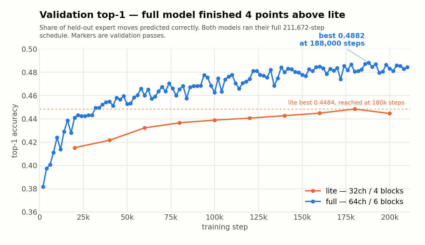
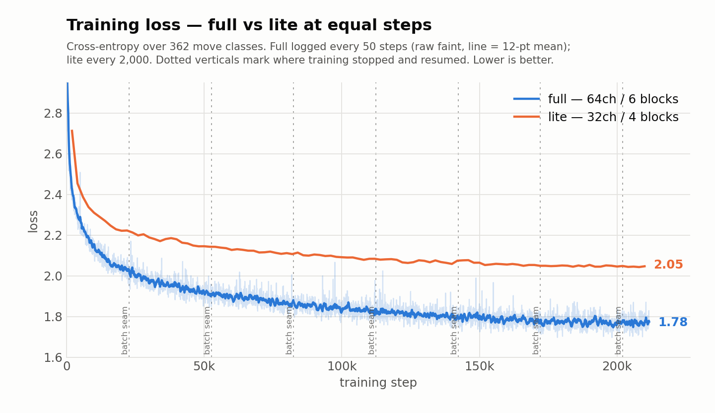
A fully-convolutional residual network trained on 138,000 games from an archive of sgf files — about 27 million positions — to predict the move a strong human actually played. The board is encoded as nine 19×19 planes (stones by colour, liberties, the last move); the output is one score per point plus a pass. Training ran on a single Nvidia GTX 1050 within ~15 hours.
Two networks ship, because size costs time in the worst possible place — inside the search loop:
| Model | Size | Top-1 | Cost per look | Used by |
|---|---|---|---|---|
| Lite | 32×4, 77k weights | 44.8% | ~1× | Gentle, Steady |
| Full | 64×6, 449k weights | 48.8% | ~6× | Thorough |
Top-1 is how often the network's first guess is the move the human actually played, on games it never saw in training. Just under half is plenty for move ordering: the search only needs the right move near the top of the list, not first. The larger network predicts better but each look costs about six times as much, out of the same clock the simulations run on — which is what decides where each one is used, below.
Those weights are a softmax. Each shape carries a learned score s, and one extra score selse stands for “none of these — play somewhere else”. The playout draws from:
Training minimises the cross-entropy of that same expression against the move the expert actually chose, so scoring and sampling are the identical formula — the table is trained on exactly the decision it is later asked to make. Sampling rather than taking the best shape is deliberate: playouts need variety, and a policy that always answered with its favourite shape would explore one line of play a thousand times instead of a thousand lines once. The selse term is what makes the softmax a choice rather than a ranking — when that share wins the draw, no local reply is played at all and the simulation falls through to a random point anywhere on the board.
Nobody has written a good way to judge a Go position by looking at it. Whether a group is alive, whether a wall outweighs a territory — these resisted hand-coding for decades, which is why computers stayed hopeless at Go long after beating the best players at chess. MCTS sidesteps the problem: instead of “how good is this position?” it asks “how often does it win?” — a question needing no Go knowledge, only the rules. That substitution took computer Go from hopeless to respectable in the mid-2000s.
Pure random play never ends sensibly, though: both sides fill their own eyes and destroy their own groups. So the simulations follow a few rules — never fill your own eye, usually answer an atari near the last move, never put a chain in atari for nothing. The search itself obeys that last rule too: a move that would join one of its own chains and leave it on a single liberty is never even considered, though a lone stone thrown into a tight spot — a real technique — still is. A chain being rescued gets a ladder check: if running it out only reaches two liberties, the escape is taken about half the time, so playouts stop chasing chains already caught. Otherwise they lean on the 3×3 shape around each empty point next to the last move — hane, cut, block, connect and the rest. Which of those shapes is worth answering, and how strongly, is learned from the same expert games as the move-prediction model: one weight per shape, trained so the point an expert actually played scores highest. Crucially it also learns when not to answer locally, which the hand-written shape library it replaced could not express — that library answered near the last move about three quarters of the time, where experts do so closer to a third. None of this is deep Go knowledge; it is just enough to make the random games plausible without slowing them down.
These control two things: thinking time, and the CNN model.
| Setting | Time / move | Network |
|---|---|---|
| Gentle | 0.26 s | Lite and Random |
| Steady | 1.5 s | Lite |
| Thorough | 6.0 s | Full |
Time decides how many loops the MCTS runs. On an ordinary laptop roughly 5,200 playouts a second on 9×9, 2,300 on 13×13 and 1,000 on 19×19.
Thorough splits the two models. One look at the Full model costs about as much as 800 playouts, so on 19×19 it is affordable exactly once — and spent at the root, where it orders the move list the whole search hangs off. Every node below it then gets the Lite model, roughly six times cheaper, which is the difference between one guided node per move and eight. On smaller boards, where evaluations are cheaper relative to the clock, the same budget reaches 18 nodes on 13×13 and 40 on 9×9.
Gentle's entry is conditional because at a quarter of a second one look can cost more than the whole move, leaving nothing to search with; the engine measures the real cost on your machine and drops the network for a random move when it would not fit. Gentle also samples loosely from its better candidates rather than always taking the most-visited move, so it is beatable without playing nonsense.
The search runs on a background thread, so the board stays responsive.
The same Monte Carlo idea, without the tree. When both players pass, the finished position is played out a couple of hundred more times and the engine watches which colour ends up owning each point. A stone standing on territory that keeps resolving to the other colour is, in practice, dead. It is a sampled guess rather than a proof, which is why you can correct any group before accepting the score.
It is strongest on 9×9, where a playout genuinely reaches the end of a real game. On 19×19 a thousand-odd simulations spread across up to 361 candidates, each playout far noisier, so the statistics firm up slowly — progressive widening and the network both narrow the search, but expect a weak-to-moderate opponent. AlphaGo's real jump in 2016 was not the policy network alone: it paired one with a value network that judges a position directly, needing far fewer simulations. This engine has no value network — every position is still judged by playing it out.
It also plays slackly when well ahead, because the simulations score only win or loss, never the margin — a two-point win counts the same as a fifty-point one, so it takes the safe, unambitious move.
Overall the goal of this program was never to design the best Go program in the world, merely a decent one that plays human moves.
The computer would rather stop than keep playing this one out.